
Big O Notation: Time Complexity, Cheat Sheet & Code Examples
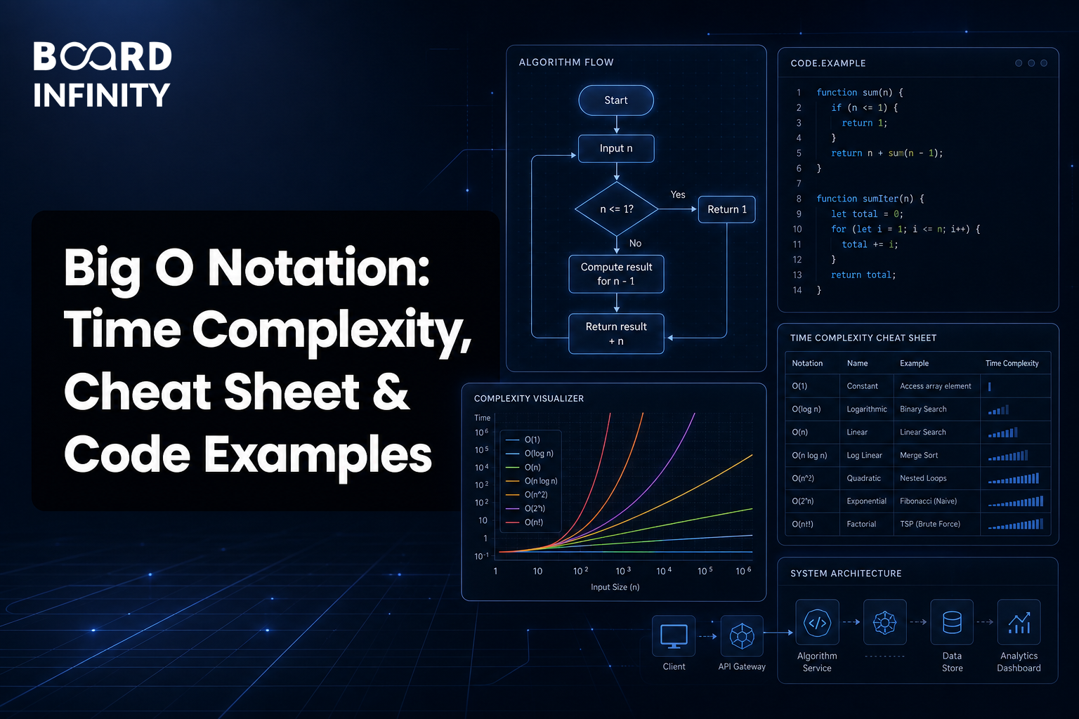
Big O notation is a mathematical way to describe how an algorithm’s running time or memory use grows as input size increases. It matters because a search that works for 100 records may fail for 10 crore records. After reading, you can compare algorithms before writing production code.
Big O sits inside algorithm analysis, along with correctness, edge cases, data structures, and implementation choices. If you are revising algorithm design basics, the relationship between steps, logic, and representation is covered in Big O Notation: Space and Time Complexity.
You will be able to identify common time complexities, simplify Big O expressions, read a big o cheat sheet correctly, and answer GATE or interview questions about loops, recursion, sorting, searching, and nested operations.
Core Concepts
Big O notation focuses on growth rate, not exact stopwatch time. The same code may run faster on one laptop and slower on another server, but its growth pattern usually stays the same. This is why interviewers ask for Big O: it shows whether your solution scales when input size grows from thousands to millions.
1.Asymptotic Bounds
Big O, Big Omega, and Big Theta are asymptotic notations. Big O gives an upper bound, Ω gives a lower bound, and Θ gives a tight bound. In interviews, candidates usually say “the time complexity is O(n)” when they mean the worst-case upper bound, but the notation itself is broader than worst case alone.
Familiar example: opening the first message in a phone inbox is O(1), while scanning all messages for a specific keyword is O(n). Industry example: a banking fraud system may guarantee at least Ω(n) work if it must inspect every transaction once, and it may be Θ(n) if it always performs exactly one pass.
Code Example
2.Simplification Rules
Big O ignores machine-specific constants and lower-order terms because growth rate dominates at large input sizes. If an algorithm takes 3n² + 10n + 50 operations, its Big O is O(n²). The n² term eventually becomes much larger than the linear and constant terms.
Familiar example: checking all pairs of photos in a gallery dominates a one-time setup step. Industry example: an e-commerce recommendation job that compares every product pair has O(n²) pair work even if it also loads a configuration file in O(1).
Code Example
3.Constant Time
O(1) means the number of operations does not grow with input size. It does not mean the operation takes one nanosecond; it means the work stays bounded by a constant. Dictionary lookup, array indexing, and reading a stack top are typical examples.
Familiar example: checking the balance shown at the top of a mobile wallet screen does not require scanning all past payments. Industry example: a PAN verification service can fetch cached metadata by PAN number using a hash map-style key lookup in expected O(1) time.
Code Example
4.Logarithmic Time
O(log n) appears when each step removes a fixed fraction of the remaining input. Binary search is the classic case: check the middle, discard half, and repeat. If the input doubles, the number of extra steps increases only slightly.
Familiar example: searching a word in a sorted dictionary by repeatedly opening the middle page. Industry example: an IRCTC-style booking system can search a sorted train-number index using binary search-like logic instead of scanning every train record.
Code Example
5.Double Logarithmic Time
O(log log n) grows even more slowly than O(log n). It appears in specialised algorithms where the index or candidate range grows extremely fast, often by repeated exponentiation or squaring. Beginners see it less often, but intermediate learners should recognise the pattern.
Familiar example: guessing a huge range where each clue lets you jump from 2 to 4 to 16 to 256 and so on. Industry example: low-level database indexing or advanced integer algorithms may use structures where lookups involve double-logarithmic terms under specific assumptions.
Code Example
6.Square Root Time
O(√n) appears when an algorithm only needs to scan up to the square root of the input value. A common example is primality testing: if n has a factor larger than √n, it must also have a matching factor smaller than √n.
Familiar example: checking whether a locker count has a divisor by testing only possible factors up to its square root. Industry example: a payment risk service may use factor-style checks or bucket decomposition where scanning √n blocks is enough instead of scanning n records.
Code Example
7.Linear Time
O(n) means the algorithm’s work grows directly with input size. If input doubles, the work roughly doubles. Single-pass validation, summation, filtering, counting, and searching an unsorted list usually fall into this class.
Familiar example: reading every item in a grocery bill to calculate the total. Industry example: a healthcare application scanning today’s appointment records to count completed consultations performs one check per appointment, so the time complexity is O(n).
Code Example
8.Linearithmic Time
O(n log n) commonly appears in efficient comparison-based sorting algorithms such as merge sort and heap sort. The algorithm has log n levels of splitting or heap adjustment, and each level processes n total elements.
Familiar example: arranging exam answer sheets by roll number using a divide-and-merge process. Industry example: an ed-tech platform sorting lakhs of leaderboard scores efficiently should prefer O(n log n) sorting over pairwise O(n²) comparisons.
Code Example
9.Quadratic Time
O(n²) appears when every item may need to be compared with every other item. Two nested loops over the same input are the usual signal. Quadratic solutions may pass for small n but become risky when n reaches lakhs.
Familiar example: comparing every guest with every other guest to find duplicate invitations. Industry example: a Zomato-style restaurant matching job that compares every restaurant with every customer preference without indexing can become O(n²)-like and expensive.
Code Example
10.Cubic Time
O(n³) appears with three nested loops over the same input size. It is common in naive matrix multiplication and some graph algorithms. Cubic time grows very quickly: increasing n from 100 to 1,000 multiplies the work by 1,000 times.
Familiar example: trying every combination of three players from a squad for a fixed role trio. Industry example: a logistics platform evaluating three-way warehouse, truck, and route combinations without optimisation may accidentally create cubic workloads.
Code Example
11.Binary Exponential Time
O(2ⁿ) appears when each input item creates two branches, usually include or exclude. This is common in brute-force subset problems. Exponential algorithms become impractical quickly because adding one more input can nearly double the work.
Familiar example: choosing all possible subsets of dishes for a party menu. Industry example: an insurance claim engine trying every combination of optional policy clauses without pruning can face exponential growth.
Code Example
12.K Way Exponential
O(kⁿ) appears when each of n positions has k choices. If k is 2, it becomes O(2ⁿ); if k is 10, the search space is much larger. This pattern appears in brute-force generation, constraint solving, and assignment problems.
Familiar example: generating all possible 4-digit numeric PINs has 10 choices for each position. Industry example: a SaaS configuration tester that tries every combination of k feature settings across n modules can become O(kⁿ) without sampling or pruning.
Code Example
13.Factorial Time
O(n!) appears when an algorithm tries every possible ordering. It grows faster than exponential time for large n. Permutation generation and brute-force travelling salesperson search are standard examples.
Familiar example: arranging all possible seating orders for a wedding table. Industry example: a courier platform that tries every possible delivery route order for n stops without dynamic programming or heuristics faces factorial growth.
Code Example
14.Independent Inputs
O(n + m) is used when an algorithm processes two independent inputs separately. Do not collapse it to O(n) unless you know m is bounded by n. This is especially common in graph problems, file merges, and multi-source data processing.
Familiar example: reading n WhatsApp contacts and m email contacts to create one combined list. Industry example: a GST invoice reconciliation job may scan n purchase records and m vendor records once each before matching through a map.
Code Example
15.Product Complexity
O(n × m) appears when every item from one input is compared with every item from another input. This is different from O(n²), where both loops usually use the same input size. Keeping variables separate makes your analysis more accurate.
Familiar example: comparing every book in one shelf with every label in another shelf. Industry example: an ONDC catalog matcher comparing n seller products with m buyer search intents without indexing performs product-sized work.
Code Example
Big O Cheat Sheet
Use this big o cheat sheet as a quick ranking from generally better to generally worse. The exact best choice still depends on constraints, constants, memory, input distribution, and correctness requirements.
- Excellent: O(1), O(log log n), O(log n)
- Usually scalable: O(√n), O(n), O(n log n)
- Risky for large n: O(n²), O(n × m), O(n³)
- Usually impractical without pruning: O(2ⁿ), O(kⁿ), O(n!)
Learning Path
Build Big O skill by analysing real code, not by memorising symbols alone. Move from simple loops to recursion, then to data structures and optimisation trade-offs.
Frequently Asked Questions
What is Big O Notation Explained with Examples for Beginners?
Big O notation explains how an algorithm’s time or space grows when input size grows. For beginners, examples such as linear search O(n), binary search O(log n), and pair comparison O(n²) make the idea concrete.
What is time complexity Big O?
Time complexity big o describes the growth rate of execution steps as input size n increases. It does not measure exact seconds because hardware, language, compiler, and network delays can change real runtime.
What is the difference between O, Ω, and Θ?
O gives an upper bound, Ω gives a lower bound, and Θ gives a tight bound. If an algorithm always makes one pass through n items, its complexity can be described as Θ(n), while O(n) is still a valid upper-bound statement.
How do I calculate Big O from code?
Count how many times the main operations run as input grows. Sequential loops are added, nested loops are multiplied, constants are dropped, and only the dominant term remains.
When is O(n log n) better than O(n²)?
O(n log n) is usually better for large input sizes because it grows much more slowly. Sorting one lakh records with an O(n log n) algorithm is far more practical than comparing every pair with O(n²).
Is O(1) always faster than O(n)?
Asymptotically, O(1) grows better than O(n), but real runtime can depend on constants and implementation details. A costly constant-time network call may be slower than a small local linear scan for tiny inputs.
What is the most common Big O mistake?
The most common mistake is treating every nested loop as O(n²) without checking loop bounds. Two loops over different inputs may be O(n × m), while a loop that halves the input each time is O(log n).
Should I mention best case and worst case in interviews?
Yes, when they differ. Linear search is O(1) in the best case if the first item matches, but O(n) in the worst case if the item is absent or at the end.
Key Takeaways
Big O notation describes growth rate, not exact runtime. O, Ω, and Θ are upper, lower, and tight asymptotic bounds. The main practical classes are O(1), O(log n), O(n), O(n log n), O(n²), O(n³), O(2ⁿ), O(kⁿ), O(n!), O(n + m), and O(n × m).
For GATE and interviews, the most tested points are simplification rules, loop addition versus multiplication, binary search as O(log n), sorting as O(n log n), pair comparison as O(n²), and recursion branching as exponential or factorial.
Further Reading
- Difference Between Algorithm and Flowchart: Definitions, Table & Examples, useful for revising algorithm representation before analysing complexity.