
CAPM, Beta & Factor Models: Interview-Ready Guide to Risk and Expected Return
Two stocks can fall 8% on the same day, but for completely different reasons. One falls because the whole market is selling off; the other falls because its own business model has cracked - CAPM and factor models are the tools that separate those two stories.
- CAPM estimates expected return as: Risk-free rate + Beta x Market risk premium.
- Beta measures systematic market sensitivity: beta above 1 moves more than the market; beta below 1 moves less.
- Diversification removes unsystematic risk, but not systematic risk - CAPM prices only the non-diversifiable part.
- Cost of equity in valuation often comes from CAPM, especially in DCF models.
- Alpha is the return left after adjusting for risk exposure; positive alpha means performance beyond the model.
- Factor models extend CAPM by adding drivers like size, value, momentum, quality and low volatility.
- Interview trap: do not say high beta means a stock is “bad”; it means it carries higher systematic risk and needs higher expected return.
Think of CAPM as a pricing lens: investors should be compensated only for risk they cannot diversify away. Factor models keep the same logic but admit that “market risk” is not the only repeated pattern in returns.
Core Explanation: CAPM, Beta and the Move to Factor Models
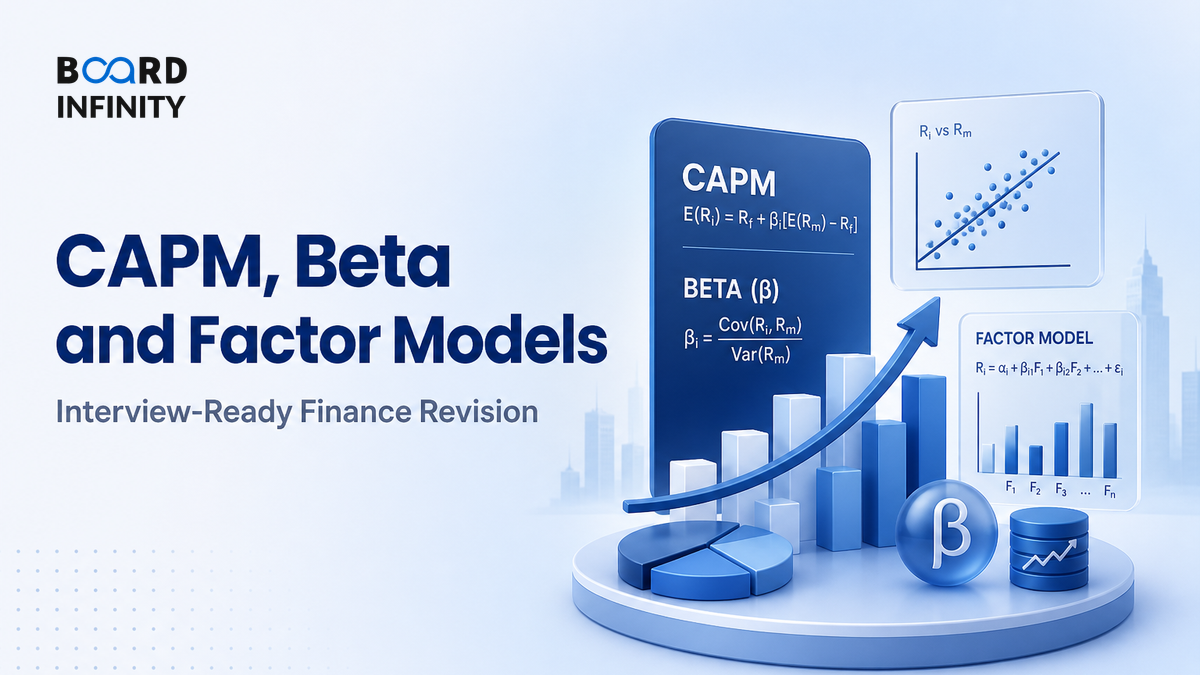
CAPM is a one-factor model. It says the expected return on an asset depends on one priced risk factor - the market portfolio. The formula is:
Expected return = Risk-free rate + Beta x Market risk premium
In symbols: Re = Rf + β(Rm - Rf), where Re is expected return or cost of equity, Rf is the risk-free rate, β is beta, and Rm - Rf is the equity market risk premium.
1. Risk-free rate: the starting line
The risk-free rate is the return investors can earn without default risk, usually proxied by a government bond yield in the same currency as the cash flows. For an Indian rupee valuation, analysts typically look at Indian government securities rather than a US Treasury rate.
2. Market risk premium: the reward for owning equities
The market risk premium is the extra return investors demand for holding the market portfolio instead of a risk-free asset. It is not the stock return itself; it is the excess return over the risk-free rate.
3. Beta: the stock’s market sensitivity
Beta answers: “If the market moves, how much does this asset usually move with it?” A beta of 1.2 means the asset has historically moved about 20% more than the market, on average, not that it will always move exactly 1.2 times on every day.
The statistical formula is:
β = Covariance(asset return, market return) / Variance(market return)
4. Cost of equity: where CAPM enters valuation
In a discounted cash flow valuation, CAPM is commonly used to estimate the cost of equity. A higher beta increases the cost of equity, which lowers the present value of future equity cash flows, all else equal.
5. Why factor models go beyond CAPM
CAPM is elegant, but markets often show return patterns not fully explained by beta alone. Factor models add more drivers: size, value, momentum, quality, profitability, investment intensity or low volatility. These models help explain why two stocks with similar market beta can still behave very differently.
Worked Example: CAPM and Alpha in 60 Seconds
Assume you are valuing an Indian listed company and using illustrative inputs:
- Risk-free rate, Rf = 7%
- Expected market return, Rm = 13%
- Market risk premium, Rm - Rf = 6%
- Stock beta, β = 1.2
Cost of equity = 7% + 1.2 x 6% = 14.2%
If the stock is expected to return 16%, then:
Alpha = Expected return - CAPM required return = 16% - 14.2% = 1.8%
Interpretation: based on these assumptions, the stock offers 1.8 percentage points more than required for its systematic risk. If the expected return were only 12%, it would look unattractive relative to its CAPM-implied hurdle rate.
Key Measures to Track
Definitions You Should Be Able to Say Cleanly
- CAPM: CAPM says expected return equals risk-free return plus beta times the market risk premium.
- Beta: Beta measures an asset’s sensitivity to market returns: covariance with the market divided by market variance.
- Systematic risk: Systematic risk is economy-wide risk that diversification cannot remove.
- Unsystematic risk: Unsystematic risk is company-specific risk that diversification can reduce or eliminate.
- Alpha: Alpha is return earned above the return predicted by the chosen risk model.
- Factor model: A factor model explains returns using multiple common drivers such as market, size, value, momentum or quality.
CAPM was developed independently by William Sharpe, John Lintner and Jan Mossin in the 1960s. The Fama-French models later popularised multi-factor explanations by adding factors such as size and value to the market factor.
Factor Models: The Practical Upgrade from Beta Alone
A factor is a broad, repeated driver of returns. Factor models are useful because two companies can have the same beta but very different exposures to profitability, leverage, interest rates, commodity prices, liquidity or momentum.
Case Study: Bajaj Finance and the Limits of One Beta
Bajaj Finance shows why analysts use CAPM as a base rate but need factor thinking to understand lending-cycle, interest-rate, regulatory and growth risks.
Situation: Bajaj Finance is one of India’s most closely watched NBFCs, operating in consumer lending, SME lending and other credit segments under RBI regulation. Its equity story is linked not only to broad market moves, but also to credit costs, funding spreads, interest-rate cycles, customer acquisition quality and digital lending compliance.
The move: When the RBI imposed restrictions in November 2023 on two digital lending products of Bajaj Finance, the issue was not simply “market beta.” It was a regulatory and process-risk event. The company worked on remedial actions, and the restrictions were later lifted in 2024. For an investor or valuation analyst, this highlighted a key point: CAPM can estimate the broad cost of equity, but scenario analysis and factor exposures are needed to understand business-specific and regulatory risks.
Outcome or lesson: Bajaj Finance’s risk profile is shaped chiefly by the credit cycle and funding environment, supported by underwriting quality, product mix, collections strength, regulatory compliance and digital execution. A shallow answer says “use beta to get cost of equity.” A strong answer says “use CAPM for the hurdle rate, then test whether additional factors can change the cash flows, valuation multiple or required return.”

How AI Changes The Capital Asset Pricing Model, Beta & Factor Models
1. Faster beta and factor estimation: AI-enabled analytics tools can pull price data, run rolling regressions and show how beta changes across calm markets, rate-hike periods or sell-offs. The student advantage is not the calculation itself, but the interpretation: why did beta rise, fall or become unstable?
2. Better qualitative factor discovery: LLMs can scan annual reports, earnings-call transcripts and regulatory filings to surface repeated risk themes - funding cost, customer concentration, commodity exposure, cyber risk, regulation or currency sensitivity. These are not always visible in historical price beta.
3. Stronger risk storytelling: Portfolio teams increasingly combine quantitative factor exposures with narrative evidence. For example, a model may show high momentum exposure, while transcript analysis may reveal margin pressure or management caution that explains why the trend may reverse.
Use NotebookLM or Perplexity to upload a company annual report, recent investor presentation and one year of price data notes. Ask: “Identify the company’s likely systematic risk factors, explain which risks CAPM captures, which it misses, and draft three interview questions on cost of equity.” Then verify every number manually before using it.
Interview Relevance
“Suppose you are valuing an Indian listed NBFC. How would you estimate its cost of equity using CAPM, and when would you prefer a factor model?”
If you remember only one sentence, use this: “CAPM gives the required return for systematic market risk; factor models explain return better when multiple systematic drivers matter.”
Common Mistake
The biggest mistake is treating beta as a label of quality - “high beta is bad, low beta is good.” That costs candidates because beta is about risk sensitivity, not business excellence. The fix: always say, “Higher beta requires higher expected return; whether it is attractive depends on price, cash flows and risk-adjusted return.”
What to Revise Next
Now move from “what return should I demand?” to “how well did the portfolio perform?” Revise Portfolio Performance: Risk-Adjusted Return Measures Explained next, especially Sharpe ratio, Treynor ratio, Jensen’s alpha and information ratio. After that, study Asset Allocation & Rebalancing, With Sample Portfolios to connect risk models with real portfolio construction.