Rider Supply, Utilisation & Delivery Time Prediction

Why does the same 25-minute delivery promise feel effortless at 4 pm and impossible at 8:30 pm? Because the problem is not just “more riders” - it is matching moving demand, moving riders, kitchen or warehouse readiness, traffic, incentives, and customer promises in real time.

Big Picture: The Operating Loop

Think of rider operations as a live control system. Demand appears in small geographic pockets, capacity must be placed before the order arrives, dispatch decisions happen in seconds, and every late order becomes training data for the next prediction.

Core Explanation: Rider Supply, Utilisation and ETA Prediction

The core idea is simple: a platform must have enough riders in the right micro-market at the right minute, while keeping each rider productively busy and giving the customer a reliable promise.

Three decisions sit on top of one another:

• Supply planning: how many riders are needed by city, zone, slot, day type, and vehicle type.
• Utilisation management: how much of rider online time is spent on active work versus waiting.
• Delivery time prediction: what time promise should be shown to the customer before and after assignment.

The 2x2 Every Candidate Should Remember

The trap is to celebrate high utilisation blindly. At 95 percent utilisation, a rider fleet may look efficient, but the next demand spike has no spare capacity. In delivery operations, a little planned slack is not waste - it is insurance against variability.

Here is how to read the matrix:

• Overstaffed stable: customers are happy, but cost per order is high because riders wait too much.
• Sweet spot: riders earn, customers receive on time, and the business controls cost.
• Idle chaos: the platform has riders, but they are in the wrong places or the dispatch logic is poor.
• Burning platform: riders are always busy, queues build up, ETAs slip, and cancellations rise.

Definitions You Must Say Cleanly

The ETA Formula: Break the Promise into Components

A strong answer never says “AI predicts delivery time” as a black box. It decomposes delivery time into operational building blocks:

A practical ETA equation is:

Predicted delivery time = preparation or picking time + rider assignment wait + rider-to-pickup travel + pickup-to-customer travel + handover buffer.

Each component has different owners. Prep time belongs to the kitchen, dark store, or seller. Assignment wait belongs to supply planning and dispatch. Travel time belongs to geography, routing, and traffic. Handover buffer belongs to building access, payment, customer availability, and packaging.

Key Metrics to Track

Use these as interview heuristics, not universal benchmarks. The right target depends on category, city density, weather, rider contracts, and the promised SLA.

A Small Worked Example

Suppose a food delivery zone expects 240 orders between 7 pm and 8 pm. Historical performance shows a rider can complete 2.4 orders per hour during this slot without hurting service level.

Base riders needed = forecast orders ÷ orders per rider hour = 240 ÷ 2.4 = 100 riders.

If the planner adds a 10 percent buffer for no-shows, rain, lift delays, and restaurant congestion, the planned supply becomes:

Final rider plan = 100 × 1.10 = 110 riders.

Now estimate ETA for one order:

• Restaurant prep time: 8 minutes
• Assignment wait: 2 minutes
• Rider-to-restaurant travel: 4 minutes
• Restaurant-to-customer travel: 12 minutes
• Handover buffer: 1 minute

Base ETA = 8 + 2 + 4 + 12 + 1 = 27 minutes. If traffic is worse than usual, add a 15 percent congestion buffer: 27 × 1.15 = 31.05 minutes. A sensible customer promise may be around 35 minutes, not 27, because the promise must survive real-world variance.

The Dispatch Cycle: Where Utilisation Becomes Customer Experience

Supply planning decides how many riders exist. Dispatch decides whether that supply becomes useful. A rider may be physically nearby but still be a poor assignment if they are carrying another order, moving away from the pickup point, unlikely to accept, or likely to miss the promise.

This is closely related to capacity balancing. If you want the manufacturing analogy, revise line balancing and workstation design: in delivery, the “workstations” are riders, kitchens, pickup points and customer locations.

Mini Case Study: Domino's India and Time-Promise Discipline

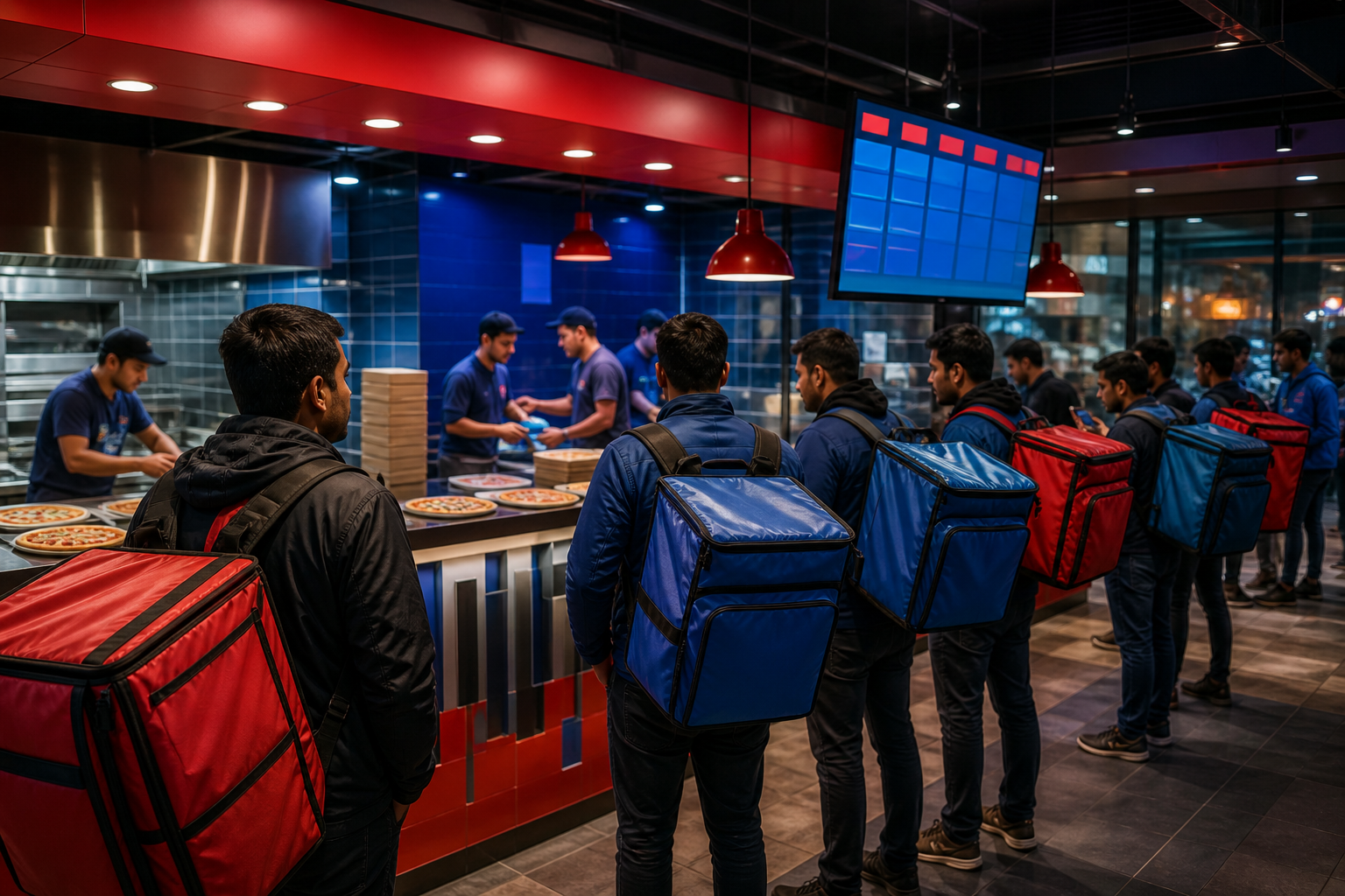
Situation. A pizza delivery business faces a tougher problem than many parcel networks: the product is time-sensitive, quality falls quickly, and the customer expectation is built around speed. The promise is not only “deliver it” but “deliver it hot, predictable, and within a familiar local radius.”

The move. Domino's India has historically relied on a dense store network, local catchment design, kitchen process discipline, and delivery execution to make the promise feasible. The primary driver is localised fulfilment from nearby stores. Supporting drivers include menu standardisation, prep-time visibility, rider staging near stores, packaging suited for short trips, and operational control over the customer promise.

The lesson. The delivery promise is not created by the rider alone. If the store is overloaded, the rider waits. If the catchment is too wide, travel time explodes. If the app promise ignores rain or peak load, the customer sees a broken SLA. Good delivery prediction is therefore a cross-functional operating system, not just a route estimate.

So what? Domino's is memorable because it proves the main point: fast delivery is designed upstream. Rider supply is only one lever; the win comes from the interaction of store density, process standardisation, local dispatch and realistic time promises.

How AI Changes Rider Supply, Utilisation and Delivery Time Prediction

AI is changing this topic in three specific ways.

• Spatio-temporal demand forecasting: models forecast orders by tiny geography and short time buckets, using signals such as weekday, rain, campaigns, holidays, local events and recent order velocity. The same logic overlaps with using AI for inventory optimisation and replenishment, where demand uncertainty also drives stocking and service decisions.
• Dynamic rider positioning and incentives: AI can identify where riders should wait before demand arrives and where temporary incentives are needed. The caution: if incentives only chase short-term supply, they can create unfair earnings volatility or train riders to wait for surge payouts.
• ETA prediction and exception detection: models estimate prep delay, travel delay, handover friction and cancellation risk, then update the promise as new signals arrive. The best systems do not only predict lateness; they trigger action before lateness becomes visible to the customer.

Interview Relevance

Common Mistake