Complete Walkthrough of AVL Trees

Complete Walkthrough of AVL Trees

Introduction

The AVL tree is a self-balancing Binary Search Tree (BST) in which there can never be more than one difference between the heights of the left and right subtrees for any given node.
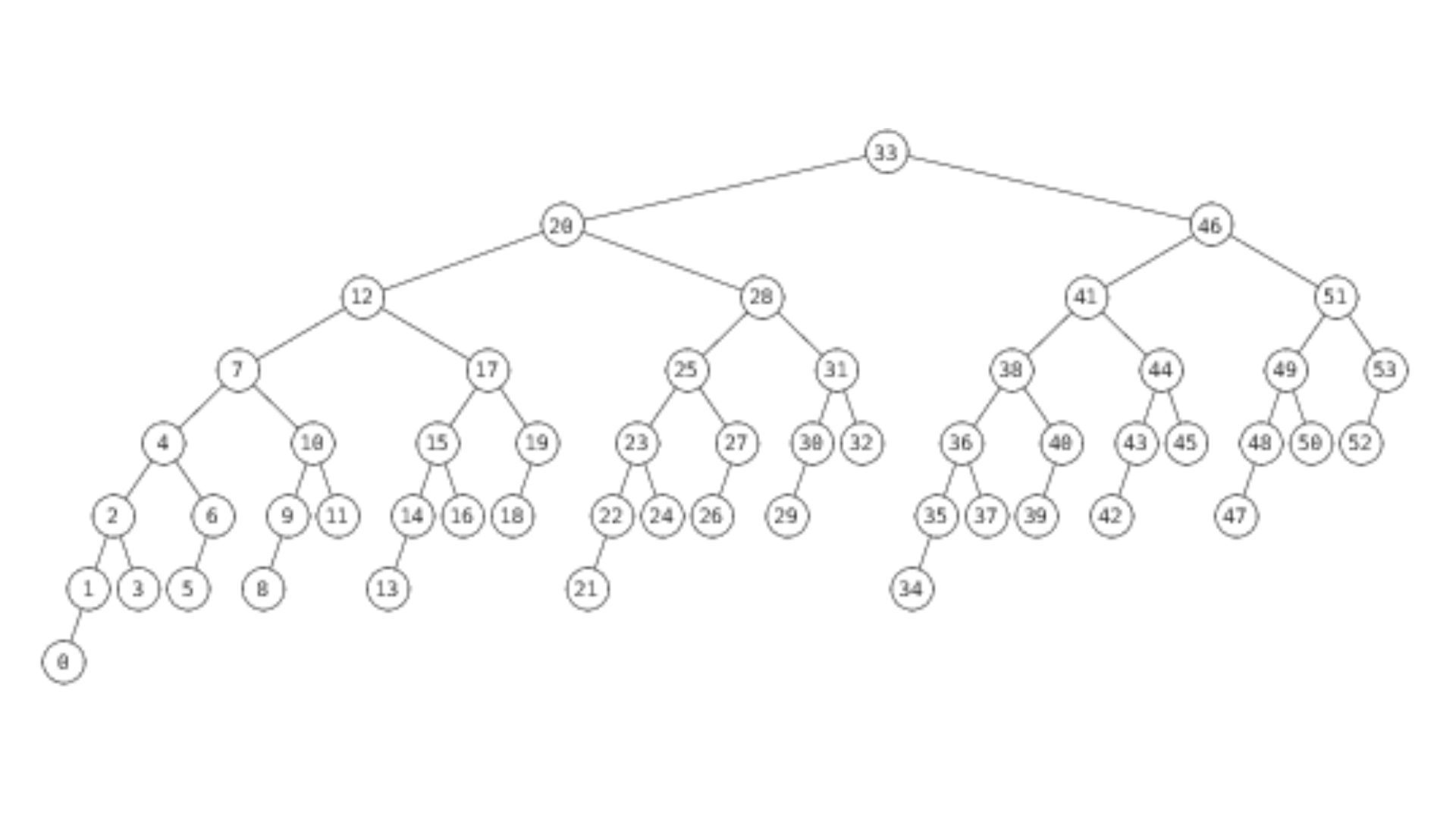
Example of AVL Tree

The heights of the left and right subtrees for each node in the above-shown tree differ by less than or equal to one, indicating that the tree is AVL.

Example of a Tree that is NOT an AVL Tree:

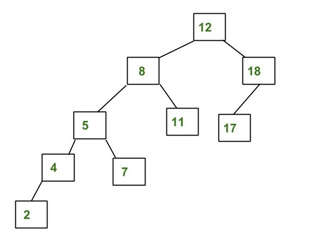
The above tree is not AVL since the left and right subtrees for 8 and 12 have height differences higher than 1.

Why AVL Trees?

Search, max, min, insert, delete, and others (e.g. of BST operation) take O(h) time, where h is the BST height. Skewed Binary trees make these operations O(n). We can ensure an upper bound of O(log(n)) for all these operations if we keep the tree height O(log(n)) after every insertion and deletion. AVL trees are always O(log(n)) with n as the number of nodes in the tree.

AVL tree insertion example

We must rebalance the BST insert process after each insertion to keep the tree AVL.

Two fundamental procedures are available for balancing a BST without violating the BST property (keys(left) < key(root) < keys(right)).

  • Right Rotation
  • Left Rotation

T1, T2 and T3 are subtrees of the tree, rooted with y (on the left side) or x (on the right side)    
     
    y                               x
    / \     Right Rotation          /  \
  x   T3   - - - - - - - >        T1   y
  / \       < - - - - - - -            / \
T1  T2     Left Rotation            T2  T3

Keys in both of the above trees follow the following order
keys(T1) < key(x) < keys(T2) < key(y) < keys(T3)
So BST property is not violated anywhere.


Steps to follow for insertion

Let’s say the newly inserted node is w.

  • Insert the standard BST for w.
  • Beginning at w, move up and locate the first unbalanced node. Let's say z is the first unbalanced node, y is its child on the path from w to z, and x is its grandchild on the path from w to z.
  • Rebalance the tree by completing the necessary rotations on the subtree whose root is z. As x, y, and z can be organized in four ways, there are four possible scenarios that must be addressed.
  • Here are the four possible arrangements:
  • Left child of z is y, while the left child of y is x. (Left Left Case)
  • Left child of z if y and the right child of y is x. (Left Right Case)
  • Right child of z is y and the right child of y is x. (Right Right Case)
  • Right child of z is y and the left child of y is x. (Right Left Case)

The operations to be conducted in the above four instances are listed below. In all circumstances, we only need to rebalance the subtree rooted with z, and the entire tree gets balanced when the height of the subtree rooted with z is the same as it was prior to insertion (after appropriate rotations).

1. Left Left Case

T1, T2, T3 and T4 are subtrees.
        z                                      y
        / \                                   /   \
      y   T4      Right Rotate (z)          x      z
      / \          - - - - - - - - ->      /  \    /  \
    x   T3                               T1  T2  T3  T4
    / \
  T1   T2

2. Left Right Case

    z                               z                            x
    / \                            /   \                        /  \
  y   T4  Left Rotate (y)        x    T4  Right Rotate(z)    y      z
  / \      - - - - - - - - ->    /  \      - - - - - - - ->  / \    / \
T1   x                          y    T3                    T1  T2 T3  T4
    / \                        / \
  T2   T3                    T1   T2

3. Right Right Case

  z                                y
\                            /   \
T1   y     Left Rotate(z)       z      x
    /  \   - - - - - - - ->    / \    / \
  T2   x                     T1  T2 T3  T4
      / \
    T3  T4

4. Right Left Case

  z                            z                            x
  / \                          / \                          /  \
T1   y   Right Rotate (y)    T1   x      Left Rotate(z)   z      y
    / \  - - - - - - - - ->     /  \   - - - - - - - ->  / \    / \
  x   T4                      T2   y                  T1  T2  T3  T4
  / \                              /  \
T2   T3                           T3   T4

Approach

The concept is to use recursive BST insert, where after insertion, we receive bottom-up pointers to each ancestor individually. Therefore, to move up, we don't require a parent pointer. The recursive code itself ascends and visits every node that was previously inserted.

To put the concept into practice, follow the steps listed below:

  • Perform the standard BST insertion.
  • The newly inserted node's ancestor must be the current node. The current node's height should be updated.
  • Find the current node's balance factor (left subtree height equal to the right subtree height).
  • If the balance factor exceeds one, the present node is unbalanced, and we are either in the Left Left or Left Right case. Compare the newly inserted key to the key in the left subtree root to determine whether it is left left case or not.
  • If the balance factor is smaller than -1, the present node is unbalanced, and we are either in the Right Right or Right-Left case. To determine whether it is the Right Right case, compare the newly inserted key to the key in the right subtree root.

The above technique is implemented as follows:

// C++ program to insert a node in AVL tree
#include<bits/stdc++.h>
using namespace std;

// An AVL tree node
class Node
{
public:
int key;
Node *left;
Node *right;
int height;
};

// A utility function to get maximum
// of two integers
int max(int a, int b);

// A utility function to get the
// height of the tree
int height(Node *N)
{
if (N == NULL)
return 0;
return N->height;
}

// A utility function to get maximum
// of two integers
int max(int a, int b)
{
return (a > b)? a : b;
}

/* Helper function that allocates a
new node with the given key and
NULL left and right pointers. */
Node* newNode(int key)
{
Node* node = new Node();
node->key = key;
node->left = NULL;
node->right = NULL;
node->height = 1; // new node is initially
// added at leaf
return(node);
}

// A utility function to right
// rotate subtree rooted with y
// See the diagram given above.
Node *rightRotate(Node *y)
{
Node *x = y->left;
Node *T2 = x->right;

// Perform rotation
x->right = y;
y->left = T2;

// Update heights
y->height = max(height(y->left),
height(y->right)) + 1;
x->height = max(height(x->left),
height(x->right)) + 1;

// Return new root
return x;
}

// A utility function to left
// rotate subtree rooted with x
// See the diagram given above.
Node *leftRotate(Node *x)
{
Node *y = x->right;
Node *T2 = y->left;

// Perform rotation
y->left = x;
x->right = T2;

// Update heights
x->height = max(height(x->left),
height(x->right)) + 1;
y->height = max(height(y->left),
height(y->right)) + 1;

// Return new root
return y;
}

// Get Balance factor of node N
int getBalance(Node *N)
{
if (N == NULL)
return 0;
return height(N->left) - height(N->right);
}

// Recursive function to insert a key
// in the subtree rooted with node and
// returns the new root of the subtree.
Node* insert(Node* node, int key)
{
/* 1. Perform the normal BST insertion */
if (node == NULL)
return(newNode(key));

if (key < node->key)
node->left = insert(node->left, key);
else if (key > node->key)
node->right = insert(node->right, key);
else // Equal keys are not allowed in BST
return node;

/* 2. Update height of this ancestor node */
node->height = 1 + max(height(node->left),
height(node->right));

/* 3. Get the balance factor of this ancestor
node to check whether this node became
unbalanced */
int balance = getBalance(node);

// If this node becomes unbalanced, then
// there are 4 cases

// Left Left Case
if (balance > 1 && key < node->left->key)
return rightRotate(node);

// Right Right Case
if (balance < -1 && key > node->right->key)
return leftRotate(node);

// Left Right Case
if (balance > 1 && key > node->left->key)
{
node->left = leftRotate(node->left);
return rightRotate(node);
}

// Right Left Case
if (balance < -1 && key < node->right->key)
{
node->right = rightRotate(node->right);
return leftRotate(node);
}

/* return the (unchanged) node pointer */
return node;
}

// A utility function to print preorder
// traversal of the tree.
// The function also prints height
// of every node
void preOrder(Node *root)
{
if(root != NULL)
{
cout << root->key << " ";
preOrder(root->left);
preOrder(root->right);
}
}

// Driver Code
int main()
{
Node *root = NULL;

/* Constructing tree given in
the above figure */
root = insert(root, 10);
root = insert(root, 20);
root = insert(root, 30);
root = insert(root, 40);
root = insert(root, 50);
root = insert(root, 25);

/* The constructed AVL Tree would be
30
/ \
    20 40
    / \  \
  10 25  50
*/
cout << "Preorder traversal of the "
"constructed AVL tree is \n";
preOrder(root);

return 0;
}

write your code here: Coding Playground

Output:

Preorder traversal of the constructed AVL tree is
  30 20 10 25 40 50

Complexity Analysis

Time Complexity: O(log(n)), For Insertion

Auxiliary Space: O(1)

Because only a few points are altered, the rotation operations (left and right rotate) take constant time. Updating the height and calculating the balance factor both take time. As a result, the AVL insert has the same time complexity as the BST insert, which is O(h), where h is the height of the tree. The height of the AVL tree is O since it is balanced (Logn). As a result, the temporal complexity of the AVL insert is O. (Logn).

Comparison with Red Black Tree

The AVL tree, as well as other self-balancing search trees such as Red Black, are handy for performing all basic operations in O(log n) time. When compared to Red-Black Trees, AVL trees are more balanced, although they may generate more rotations during insertion and deletion.

Therefore, if your application requires frequent insertions and deletions, Red Black trees should be used. And, if insertions and deletions are rare and searching is the most common activity, the AVL tree should be preferred over the Red Black Tree.