Branch And Bound Algorithm: Explained
Branch and Bound (B&B) is one of the most effective heuristic approaches for solving different kinds of optimization problems to be found in the domain of Operations Research and Computer Science. It is a finite algorithm, that is, it provides a solution to a problem, unlike heuristic algorithms which provide approximate solutions. This algorithm is useful in solving problems including the TSP, Integer linear programming, Knapsack problem, and others.
What is Branch and Bound?
Branch and Bound is an optimization algorithm with a general application to decision problems that require a solution presentable in the form of a structure and where the structure can be partitioned into substructures. Branch and bound function in computation is done by breaking down the problem under consideration into subproblems, estimating the potential solutions using bounds, and excluding parts of the search space that will not contain an optimal solution.
Key Concepts in Branch and Bound
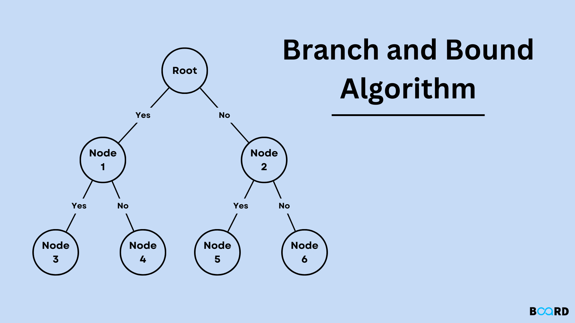
Branching: This is the process of sharing the problem with a number of other simpler problems that are easier in terms of solving. All the subproblems are potential solutions to the main problem. These subproblems are usually created by taking sequences of decisions to find how to transform the big problem into smaller and more easily solvable ones.
Bounding: After that, when a subproblem is produced, the next step is to assess the feasibility of the best solution for this particular subproblem. This is done by calculating a bound - upper or lower bound for the solution. If the bound calculated suggests that the subproblem cannot find a better solution than an already known solution, it is excluded.
Steps of the Branch and Bound Algorithm
Step 1: Initialization
This is the first step to formulate the problem by identifying the sense in which the thing is being optimized, the constraints that have to be faced, and what constitutes a solution in the set of all admissible solutions. The first step is normally the best solution obtained for now and it’s normally infinity or any other known initial solution.
Step 2: Branching
It is then partitioned into subproblems by decisions that bring out branches in the search space. This is the branching phase, where the solution space is divided based on some criterion. More specifically, this is the phase that sees the solution space split along one or more dimensions depending on some criteria - Sub Branching more precisely - a phase where the branching is done and the solution space is split along one or more dimensions depending on a criteria Sub Branching. For instance, in the Traveling Salesman Problem (TSP), a branch can choose the next city to visit.
Step 3: Bounding
In correspondence with each of the subproblems created by branching, an appraisal is determined. The bound gives information about the optimality or the quality of the solution which one may get from that subproblem. The bound can be either:
✅Upper Bound: Optimal solution from the subproblem that can be attained in scenarios in which we need to minimize the objective function.
✅Lower Bound: A solution that is worst possible from the subproblem and used where the aim is to maximize the objective function.
Step 4: Pruning
If the bound of a subproblem is worse than the bound of the best solution caned so far, then that branch cannot be pursued so the algorithm does not follow that path. This process of pruning is very important to cut the search space.
Step 5: Repeat
This is the case in the algorithm where the branching, bounding, and pruning go round and round until no further subproblem is to be undertaken. This is the optimum solution current best solution based on evaluations done throughout this process.
Step 6: Termination
When all branches are fully traversed or cut, the algorithm ends its operations execution process, and then it is complete. The best solution among those observed within the course of execution is returned as the final solution.
Classification of Branch and Bound Algorithms
Branch and Bound is a versatile algorithm as it can be employed in various types of problems. There are two common approaches for implementing Branch and Bound:
a) Best-First Search
Here the selection process is used because the algorithm always selects the subproblem that has the lowest bound. Unlike max-heap, min-heap, or priority queue, it holds the subproblems in the order of their bounds. This method is employed most commonly when we want to organize the search process in a way that permits us to come across the initially promising subproblems.
b) Depth-First Search
In this approach, the algorithm works as deeply as possible along one branch in the search space formed and then goes back and branches out on another branch. This method can be more memory-efficient for a similar reason – no priority queue needs to be stored. It is commonly applied where memory is going to be a big issue.
Benefits of Branch and Bound Algorithm
- Exact Solution: Branch and Bound assures you of finding the best solution while heuristics at best give you a sub-optimal solution.
- Efficiency: It reduces the options in which the process searches for the required solution by eliminating those that are closely left to other options hence becoming efficient.
- Flexibility: It can be used to solve issues that seek to minimize or maximize an answer to any given problem.
Disadvantages of Branch and Bound Algorithm
- Computational Complexity: Branch and Bound can still become relatively costly for large problem spaces because, despite pruning, it has to explore a large part of the search space.
- Memory Usage: Using all the branches and bounds might consume a huge amount of memory, most notably for large problems.
- Slow for Large Problems: Branch and Bound may require a lot of time to come up with an optimum solution if the domain search space is large and the bounds are not that effective in eliminating hopeless branches.
Example of Branch and Bound: Solving the Knapsack Problem
Now let’s look at the basic idea behind what is called the 0/1 Knapsack Problem. Our constraint is a knapsack with a capacity of 50 units that should be filled to make the most of the value of the items that can fit in it. In other words, the goal is to choose items whose combined weight does not exceed 50 units and, at the same time provide the chance to get the maximum value.
✅ Step 1: It is good to begin the evaluation by considering the maximum value that the subproblem can assume based on the limitations in place.
✅ Step 2: Expand the branches by thinking of whether or not each item should be included or excluded in the knapsack.
✅ Step 3: For any branch compute the bound, and cut-off branches that cannot produce a better solution than the one being worked on currently.
✅ Step 4: Proceed until all branches of the tree are emptied or cut off as part of a decision-making process.
By doing this the Branch and Bound technique will arrive at the right combinations of items to include in the knapsack.
Conclusion
Branch and Bound is one of the impressive and flexible approaches to solving combinatorial optimization problems. In fact, it becomes most valuable when the space of problems is large and straightforward searches are too time-consuming. Branch and Bound works correctly because it divides a problem into subproblems and uses bounds to rule out unfruitful search spaces. Nevertheless, for extremely large problems, the algorithm faces some issues because of the exponentially increasing investigation area and bound optimization is an essential prerequisite for the solution’s efficiency.