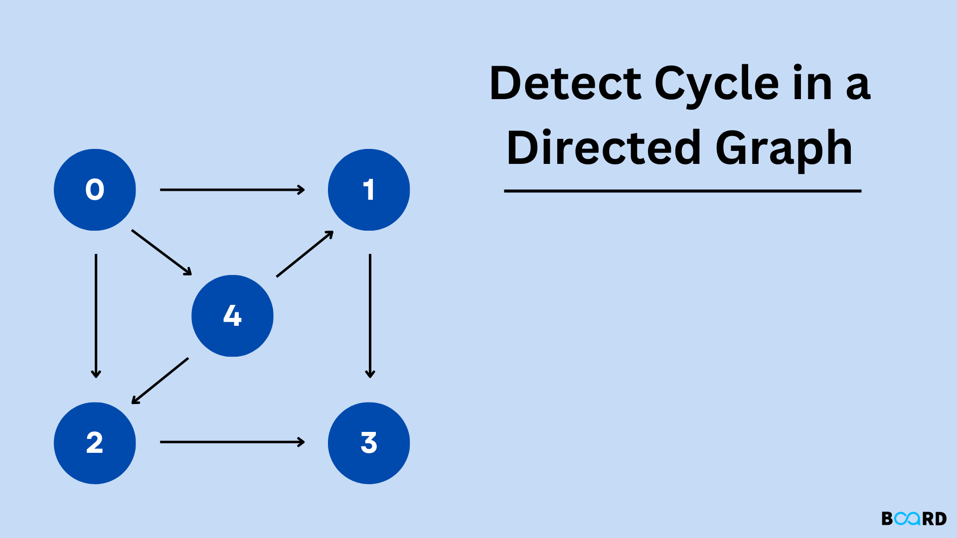
Detect Cycle in Direct Graph
Introduction
In real-world applications, directed graphs are typically used to represent a set of dependencies. A course prerequisite in a class schedule, for example, can be represented using directed graphs.
And cycles in this type of graph indicate deadlock — in other words, doing the first task requires waiting for the second, and doing the second requires waiting for the first. Detecting cycles is therefore critical in order to avoid this situation in any application.
Problem Explanation
We want to find cycles in a directed graph. These cycles can be as simple as one vertex connected to itself or as complex as two vertices connected as illustrated:

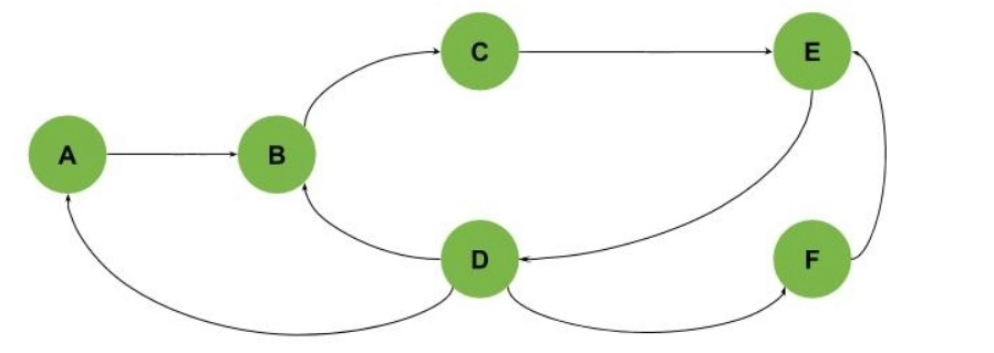
Or we can have a larger cycle, as shown in the following example, where the cycle is B-C-D-E:

We can also get graphs with multiple intersecting cycles, as shown (we have three cycles: A-B-C-E-D, B-C-E-D, and E-D-F):
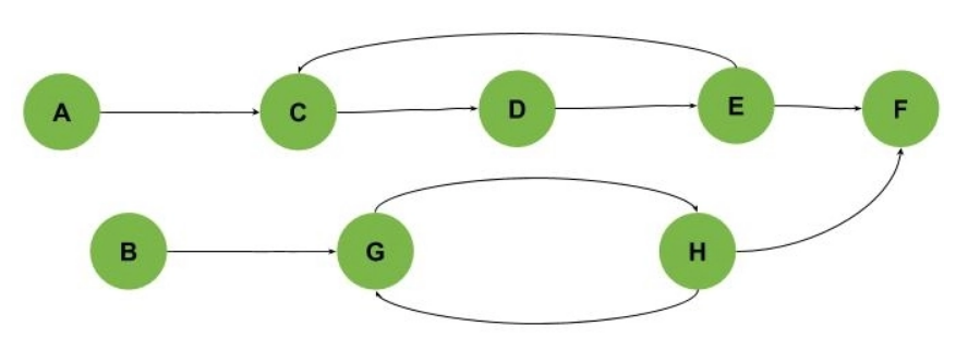
It's also worth noting that in all previous examples, we can find all cycles by traversing the graphs from any node. This is not the case in all graphs.
In some graphs, we must begin visiting the graph from various points to find all cycles, as shown in the following example (Cycles are C-D-E and G-H):
Algorithm Idea
It is simple to find cycles in a simple graph, as shown in the first two examples in this article. We can traverse all of the vertices and see if any of them are connected to themselves or to another vertex that is connected to them. Of course, this will not work in more complex scenarios.
Depth-First-Search is a well-known method for locating cycles (DFS). DFS Trees are created by traversing a graph using DFS. The DFS Tree is essentially a reorganisation of graph vertices and edges. And, after constructing the DFS trees, we have classified the edges as tree edges, forward edges, back edges, and cross edges.
Let's look at an example from our second graph:

In the previous example, we can see that the edge E-B is labelled as a back edge. A back edge is an edge in the DFS Tree that connects one of the vertices to one of its parents.
The edge A-C is also marked as a forward edge in the previous example. A forward edge connects a parent to one of the DFS tree's non-direct children.
In our graph, you'll notice that the normal edges are also represented by solid lines. The tree edges are represented by these solid line edges. The tree edges are defined as the main edges visited to construct the DFS tree.
Let's look at another example with multiple back edges:

We can identify cycles in our graph with each back edge. So, by removing the back edges from our graph, we can obtain a DAG (Directed Acyclic Graph).
Let's look at one more example to illustrate another problem we might encounter:

In this final example, an edge is labelled as a cross edge.
To understand this section, consider the DFS over the given graph. If we begin the DFS on this graph at vertex A, we will visit vertices A, C, D, E, and F.
Still, we won't be able to see the vertices B, G, and H. So, in this case, after the first run, we must restart the DFS from a different point that was not visited, such as vertex B. We'll have multiple DFS Trees as a result of these multiple DFS runs.
A single graph can have multiple DFS trees. In our example, the cross edge is the vertex connecting one of the DFS trees in our graph to another DFS tree.
If a cross edge does not connect a parent and child, it can exist within the same DFS tree (an edge between different branches of the tree).
Flow Chart
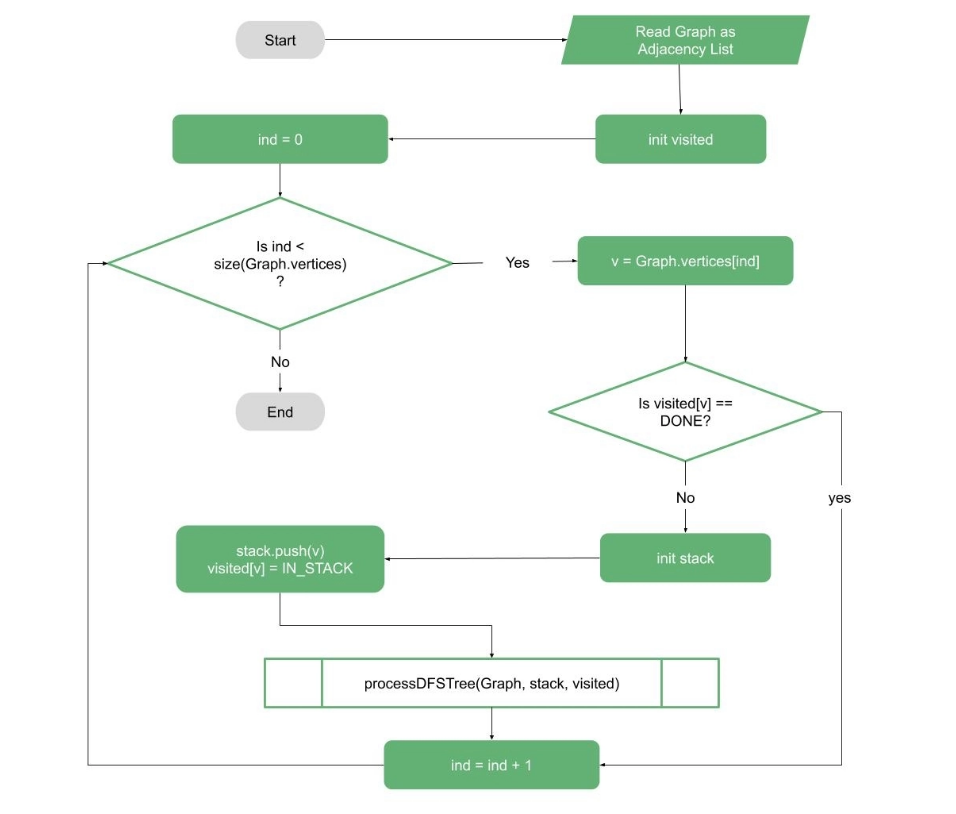
The main idea can be illustrated simply as a DFS problem with some modifications. The first step is to ensure that the DFS is repeated from each unvisited vertex in the graph, as shown in the flowchart below:
The DFS processing is the second part. In this section, we must ensure that we have access to the DFS stack in order to check for back edges.
And we know we've found a cycle (or multiple cycles) when we find a vertex that is connected to another vertex in the stack:

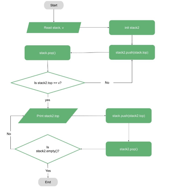
If we want to print the first cycle, we can use the flowchart below to do so using the DFS stack and a temporary stack:
However, if we want to convert the graph to an acyclic graph, we should avoid printing the cycles (as printing all cycles is an NP-Hard problem).
Instead, we should mark and remove all of the back edges in our graph.
Pseudocode
The following section of this tutorial will provide a simple pseudocode for detecting cycles in a directed graph.
The input to this algorithm is a directed graph. For the sake of simplicity, we'll assume it's using an adjacency list.
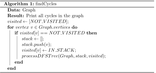
The first function is an iterative function that reads the graph and generates a list of flags for graph vertices that are initially marked as NOT VISITED (called visited in this pseudocode).
The function then iterates through all of the vertices, calling the function processDFSTree whenever it encounters a new NOT VISITED vertex:
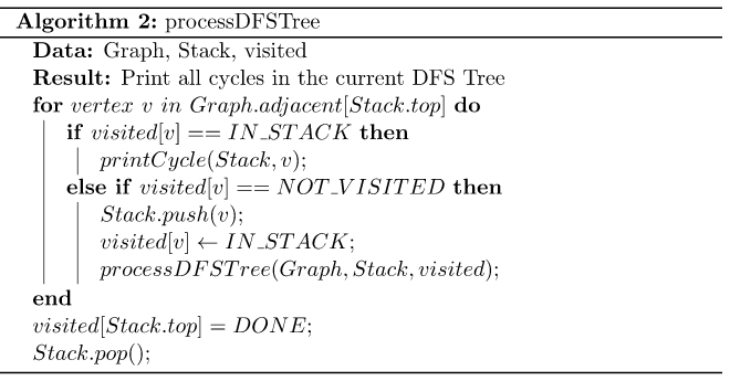
The recursive function processDFSTree takes three inputs: the graph, the visited list, and a stack. Following that, the function primarily performs DFS, but it also marks the discovered vertices as IN STACK when they are discovered.
And once the vertex has been processed, we mark it as DONE. If we find a vertex that is IN STACK, we have discovered a back edge, which indicates that we have discovered a cycle (or cycles).
As a result, we can print the cycle or mark the back edge as follows:
Let's finish by writing the function that prints the cycle:

The printing function primarily requires the stack and the vertex discovered with the back edge. The function then pops the elements from the stack and prints them before pushing them back with the help of a temporary stack.
Complexity
The given algorithm's time complexity is primarily the DFS, which is O(|V| + |E|).
In terms of space complexity, we need to allocate space for marking the vertices as well as the stack, so it will be in the order of O(|V|).
Conclusion
We covered one of the algorithms for detecting cycles in directed graphs in this tutorial. We began by discussing one of the algorithm's most important applications. Then, using examples, flowcharts, and pseudocode, we explained the concept and demonstrated the general algorithm concept.